3D acquisition techniques: Structure from Motion

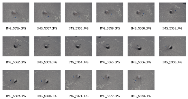
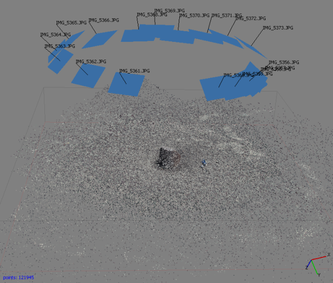
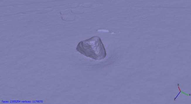
Structure from Motion (SfM), also known as Multi-View Stereo (MVS), is a technique for creating three-dimensional digital models from a set of photographs. Fundamentally, it is a stereo vision approach, that is, it uses the parallax (the difference in the apparent relative position of an object if seen from different directions) to derive 3D information (distance/depth) from 2D images. (Look at something that has foreground and background, e.g. a plant on your window sill and the house on the other side of the street, alternate between your right and left eye – the shifts you see is the parallax.)

What you need for SfM is several (2, 3, … thousands) photographs capturing an object from many different directions. Then, there are by now several software products that can perform SfM 3D reconstruction. VisualSfM (open source) and Agisoft Photoscan ($179 standard, $3499 professional) appear to be among the more popular solutions. There are several more, and there are quality, speed and usability differences, but essentially they all do the same.

A series of photographs of a rock in the desert.

The software will first analyse the photographs to find many (usually several thousand) characteristic feature points within each image, using SIFT (Scale-Invariant Feature Transform) or similar algorithms. The feature points are defined by analysing the surrounding pixels which will help to recognise similar feature points in other images. Algorithms like SIFT (rather than just trying to directly match small regions among images, e.g. by correlation) ensure that this works irrespective of scale or rotation.

The next step is to match these feature points among images to find corresponding feature points. Some feature points will not be found in any other image – so what, there are many more. Some others will be mismatched, so outliers will be recognised and excluded. The next step is the actual heart of the SfM approach: bundle adjustment. The theory for this has been around for decades, but only with powerful computer hardware was it possible to actually do this (who wants to do billions of computations on a piece of paper…). What happens during bundle adjustment is that the software tries to find appropriate camera calibration parameters and the relative positions of cameras and the feature points on the object. It is quite a challenging optimisation problem, but after all its not magic but just very sophisticated number crunching.

The algorithm starts by using two images. It assumes the known camera focal length (from the JPG’s EXIF data) or (if no data are available) a standard lens. It then uses the relative (2D) positions of the feature points in the two images to derive a rough estimate of the 3D coordinates of these points relative to the camera positions, then iteratively refines both the camera parameters and the 3D point coordinates until either a certain number of iterations or a certain threshold in the variance of the point positions has been reached. Then, the next image is added, and the software tries to fit the matched feature points of that image into the existing 3D model, iteratively refines the parameters and so on. After all images have been added, an additional bundle adjustment is run to refine the entire model. And then, voilá, there’s your sparse 3D point cloud and your modelled camera calibrations and positions.

Sparse point cloud with modelled camera positions.

Now, there are three or four things still worth considering. One is that you may observe slight differences in modelled camera calibration parameters or 3D data. That’s a relatively common issue when dealing with iteratively optimised data. What comes out of the process is not the “absolute truth” but something that is usually quite close to it.

The second point is that the 3D model somehow floats in space – it is not referenced to any coordinate system. Depending on the software, referencing can be done directly by inserting control points with known positions or by using known camera positions as control points. Alternatively, referencing can be done in external software (for example by applying a coordinate transform to the point cloud using Java Graticule 3D. For some purposes, the non-referenced model is good enough, for others you might at least want to scale it, for yet others a complete rotate-scale-translate transformation to reference the model to a coordinate system is necessary.

The third point is that you may want a denser point cloud. To get this, software like VisualSfM or Agisoft Photoscan uses the camera positions, orientation and calibration together with the sparse point cloud and the actual images to compute depth (distance) maps: for every pixel in the image (but usually resampled to a lower resolution), the distance between camera and object is computed. From these distance maps, a dense point cloud is then created.

Finally, what if you need a meshed model? It is either created directly after dense point cloud generation (Agisoft Photoscan), or meshing can be done in external software.

Meshed model of the rock in the desert.